Convenience Tools
sdss_brain offers starter tools, based off the Brain, that can be further customized and subclassed
to enable enhancements specific to the science domain.
Note
These tools are not meant to be final science-ready tools and products. They are meant to be subclassed, customized, and improved with mapper-, survey-, science-specific functionality and features.
Spectral Data
For spectral data, the Spectrum helper class exists that loads underlying spectral data. A few starter
tools are currently available for SDSS spectral data. Available sub-tools are:
Eboss: single fiber SDSS BOSS / EBOSS spectraMangaCube: SDSS Manga IFU data cubesApStar: SDSS APOGEE-2 combined spectra for a single starApVisit: SDSS APOGEE-2 single visit spectra for a given starAspcapStar: SDSS APOGEE-2 combined stellar spectra with ASPCAP results
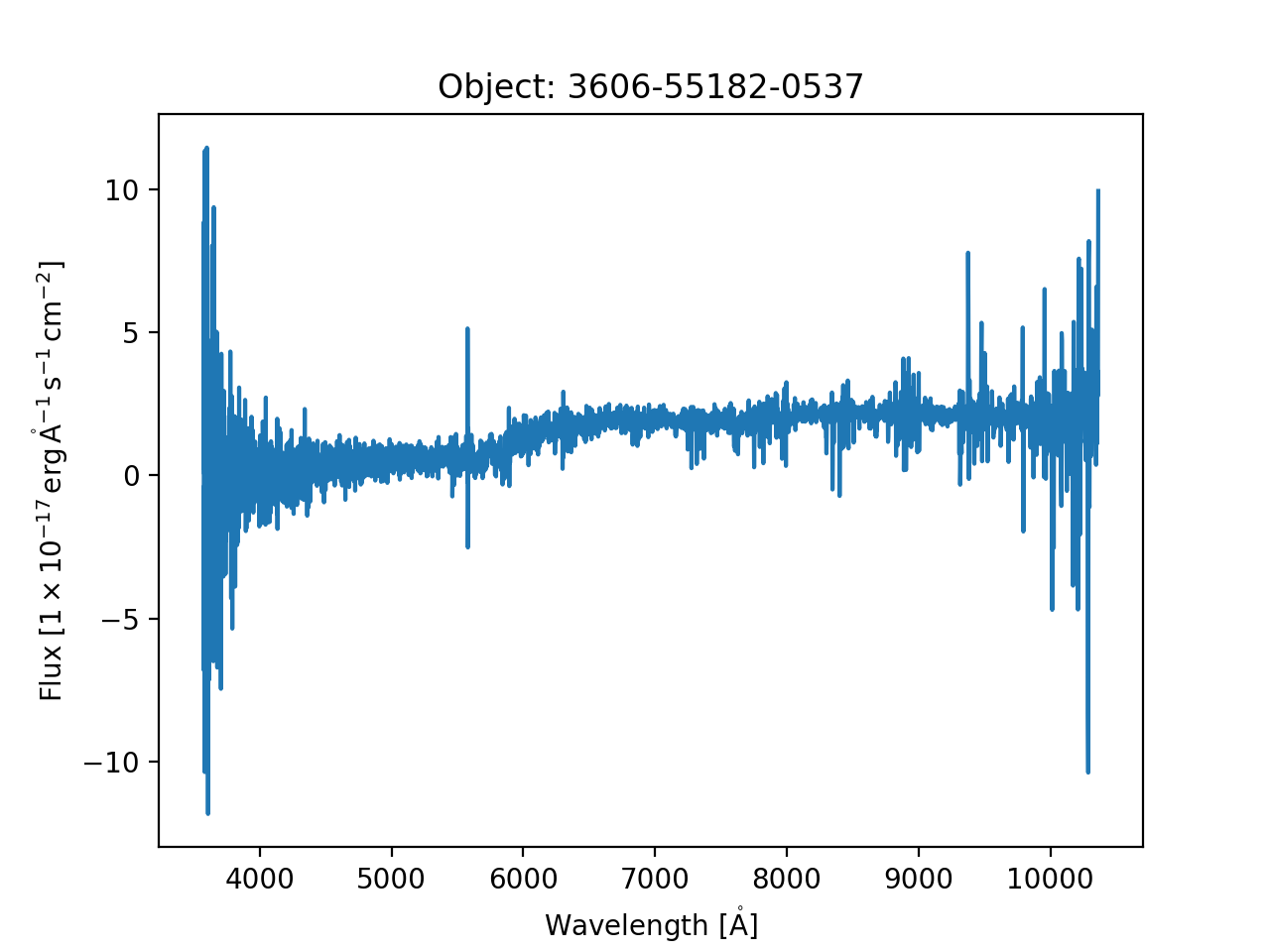
Let’s load a single fiber EBOSS spectrum from plate 3606, mjd 55182, fiber 0537 from the DR14 public data release.
>>> # load a single fiber Eboss spectrum
>>> from sdss_brain.tools import Eboss

>>> objid = '3606-55182-0537'
>>> e = Eboss(objid, release='DR14')
>>> e
<Eboss objectid='3606-55182-0537', mode='local', data_origin='file', lite=True>
If the data has been loaded from a file, the full HDUList is available as the data attribute.
The FITS header also gets loaded into a header attribute.
>>> # display the FITS data and header
>>> e.data.info()
Filename: /Users/Brian/Work/sdss/sas/dr14/eboss/spectro/redux/v5_10_0/spectra/lite/3606/spec-3606-55182-0537.fits
No.    Name      Ver    Type      Cards   Dimensions   Format
0  PRIMARY       1 PrimaryHDU     125   ()
1  COADD         1 BinTableHDU     26   4626R x 8C   [E, E, E, J, J, E, E, E]
2  SPALL         1 BinTableHDU    488   1R x 236C   [27A, 14A, 4A, E, E, J, J, E, J, E, E, E, K, K, K, K, K, K, K, K, K, B, B, J, I, 5E, 5E, J, J, J, J, 7A, 7A, 16A, D, D, 6A, 21A, E, E, E, J, E, 24A, 10J, J, 10E, E, E, E, E, E, E, J, E, E, E, J, 5E, E, E, 10E, 10E, 10E, 5E, 5E, 5E, 5E, 5E, J, J, E, E, E, E, E, E, 16A, 9A, 12A, E, E, E, E, E, E, E, E, J, E, E, J, J, 6A, 21A, E, 35E, K, 19A, 19A, 19A, B, B, B, I, 3A, B, I, I, I, I, J, E, J, J, E, E, E, E, E, E, E, E, 5E, 5E, 5E, 5E, 5E, 5E, 5E, 5E, 5E, 5E, 5E, 5E, 5E, 5E, 5E, 5E, 5E, 5E, 5E, 5E, 5E, 5E, 5E, 5E, 5E, 5E, 5E, 5E, 5E, 5E, 5E, 5E, 5E, 5E, 5E, 5J, 5J, 5J, 5E, 5J, 75E, 75E, 5E, 5E, 5E, 5J, 5E, D, D, D, D, D, D, D, D, D, 5E, 5E, 5E, 5E, 5E, 5E, 5E, 5E, 5E, 5E, 5E, 5E, 5E, 5E, 5E, 5E, 5E, 5E, 5E, 5E, 5E, 5E, 5E, 5E, 5E, 5E, 5E, 5E, 5E, 5E, 5E, 5E, 5E, 5E, 5E, 5E, 5E, 5E, 5E, 5E, 5E, 5E, 40E, 40E, 5J, 5J, 5E, 5E, 5D, J, J, J, J, J, J, J, E]
3  SPZLINE       1 BinTableHDU     48   32R x 19C   [J, J, J, 13A, D, E, E, E, E, E, E, E, E, E, E, J, J, E, E]

>>> e.header
SIMPLE  =                    T / conforms to FITS standard
BITPIX  =                    8 / array data type
NAXIS   =                    0 / number of array dimensions
EXTEND  =                    T
TELESCOP= 'SDSS 2.5-M'         / Sloan Digital Sky Survey
FLAVOR  = 'science '           / exposure type, SDSS spectro style
BOSSVER = 'branch_jme-rewrite+svn105958' / ICC version
MJD     =                55182 / APO MJD day at start of exposure
MJDLIST = '55181 55182'        /
RA      =            28.001011 / RA of telescope boresight (deg)
DEC     =             0.000273 / Dec of telescope boresight (deg)
...
The class has built-in support for spectral data using
specutils. If specutils supports the specific file
format, it automatically reads in the data to a Spectrum1D object, which is a fully represented
NDData object. See the specutils documentation
for more information on what you can do with a Spectrum1D object.
>>> # access the spectrum1D data
>>> e.spectrum
<Spectrum1D(flux=<Quantity [-1.3572823 , -0.40395638, -6.811142  , ...,  3.6619325 ,
        2.775676  ,  9.941529  ] 1e-17 erg / (Angstrom cm2 s)>, spectral_axis=<SpectralCoord [ 3572.7283,  3573.552 ,  3574.374 , ..., 10358.569 ,
            10360.958 , 10363.348 ] Angstrom,
    radial_velocity=0.0 km / s,
    redshift=0.0,
    doppler_rest=0.0 Angstrom,
    doppler_convention=None,
    observer=None,
    target=None>, uncertainty=StdDevUncertainty([6.29442  , 6.3023944, 6.259549 , ..., 4.1046424,
               3.6570566, 3.1807606]))>
The Spectrum lets you quickly plot a spectrum to display as a matplotlib plot.
# plot the spectrum object
e.plot()
Currently there is no SDSS API yet. However, all tools work remotely by using
load_from_url, a function that streams the file via an HTTP get request and loads
its contents into an in-memory FITS object. Let’s load a different EBOSS spectral fiber, 550, one
that we may not have locally.
>>> # load eboss fiber 550 remotely
>>> e = Eboss('3606-55182-0550', release='DR14')
>>> e
<Eboss objectid='3606-55182-0550', mode='remote', data_origin='api', lite=True>

>>> e.spectrum
<Spectrum1D(flux=<Quantity [ 8.872343  ,  0.41632798, -4.9438033 , ...,  1.0025655 ,
        -1.176005  ,  8.128782  ] 1e-17 erg / (Angstrom cm2 s)>, spectral_axis=<SpectralAxis [ 3571.9065,  3572.7283,  3573.552 , ..., 10358.569 , 10360.958 ,
10363.348 ] Angstrom>, uncertainty=InverseVariance([0.00840226, 0.01222116, 0.01264216, ..., 0.04095282,
                0.05368033, 0.06472613]))>
Context Managers
The Brain and all subclasses act as open data handlers. For example, they open FITS data and make it
directly accessible via the data attribute. Each tool or Brain subclass comes with a
destructor method that should safely close any open files, database connections, or remote request
sessions. Alternatively you can use each tool as a contextmanager to safely access underlying data.
with Eboss(s, release='DR14') as e:
    spectrum = e.spectrum